There is a growing interest in applying machine learning techniques on medical data. Brain scans from Magnetic Resonance Imaging experiments (MRI) have been a popular choice with the number of…

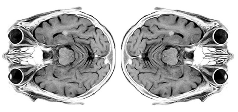Structural MRI scan of the human brain (modified from toubibe)

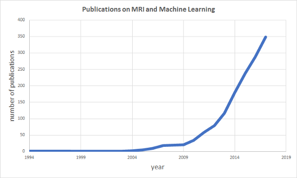
There is a growing interest in applying machine learning techniques on medical data. Brain scans from Magnetic Resonance Imaging experiments (MRI) have been a popular choice with the number of publications combining MRI and machine learning growing exponentially over the last years (see data from PubMed below). Therefore in this first post we will cover some of the basics about structural and functional MRI (fMRI) data to give you an idea of how the data is generally structured. In the following post we will analyze the data by doing some correlation analysis and by building a general linear model (GLM) to identify active regions in the brain.

The focus of these posts will be on the structure and analysis of the data and not on the underlying principles of magnetic resonance imaging.

Structural MRI  images

Structural MRI scans usually visualize the location of water in the human body. This means that soft tissues with high water and fat concentration such as the brain can be well resolved while more dense structures such as bones have a lower signal amplitude. Structural MRI scans allow clinicians to visualize and locate anatomical structures within the brain in great detail. This is why fMRI experiments which try to identify active regions in the brain during specific tasks are typically combined with structural MRI scans. Although structural MRI images are often shown as 2-D images they actually represent volume information. That is why the elements in each image are referred to as volumetric pixels, or voxels, instead of pixels as in standard 2-D images. Typically the brain is scanned in several planes or slices during a MRI session which underlines the volumetric nature of the method. We will see later when we come to functional MRI scans (fMRI) what this means in practice.

The Dataset

The data for this project can be either downloaded manually from the SPM homepage or you can use the code in the Jupyter Notebook for this post which takes care of downloading and unzipping the data. SPM is a popular Matlab toolbox for analyzing fMRI experiments. The data we are going to use here is from a human subject laying in a MRI machine while listening to “ bi-syllabic words” as the description reads on the SPM homepage. This auditory stimulation will later allow us to see which areas in the brain are involved in perceiving these words. But first we will have a look at the structural MRI scan.

Visualizing structural MRI data

After loading in the data with the help of the NiBabel library we can see that the data actually has 4-Dimensions. The first two are the X- and Y-planes while the 3rd dimension represents the number of slice in the scan. The 4th dimension does not contain any information and can be discarded.

>>> print(data.shape)  
(256, 256, 54, 1)

The output above tells us that the brain was scanned in 54 slices with a resolution of 256 x 256 voxels per slice. In order to visualize each slice we need to rearrange the data.

>>> import numpy as np  
>>> data = np.rot90(data.squeeze(), 1)  
>>> print(data.shape)  
(256, 256, 54)

Applying the above code removes the 4th empty dimension of the dataset and rotates each slice so that the eyes are facing upwards when plotting the images in the next step. Because 54 slices are a bit too much to display at once we will only plot every 10th slice here.

>>> import matplotlib.pyplot as plt  
>>>  
>>> fig, ax = plt.subplots(1, 6, figsize=[18, 3])  
>>>  
>>> n = 0  
>>> slice = 0  
>>> **for** _ **in** range(6):  
>>>     ax[n].imshow(data[:, :, slice], 'gray')  
>>>     ax[n].set_xticks([])  
>>>     ax[n].set_yticks([])  
>>>     ax[n].set_title('Slice number: **{}** '.format(slice), color='r')  
>>>     n += 1  
>>>     slice += 10  
>>>      
>>> fig.subplots_adjust(wspace=0, hspace=0)  
>>> plt.show()

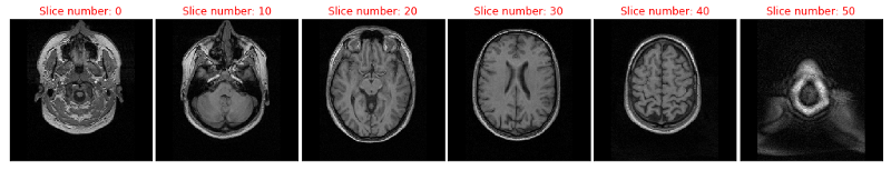
Alright this looks like a brain in a skull. For your orientation we are looking at the subjects brain from the top with slice 0 being the lowest one and slice 50 the highest one. In slice 20 you can see the eyes. Next we will look at the second part of the dataset, the fMRI data.

Functional MRI images

While structural MRI images provide a lot of spatial detail about the brain or other organs under investigation functional MRI, or fMRI, scans monitor the blood-oxygen-level dependend signal (BOLD signal) over time, which comes at the expense of loosing spatial detail. Essentially the BOLD signal represents changes in the blood oxygenation of brain tissue which can be used as an indirect measure of brain activity but is NOT an equivalent of neural activity.

Visualizing functional MRI data

So now lets have a look at the functional data. First we open the README.txt that comes with the dataset because here the details of the data acquisition are documented. We need these not only to read the fMRI files but also to make sense out of the data later on. The key parameters for now are the size of each image (64 x 64 voxels), the number of slices that were collected (64) and how many volumes were acquired (96); that is the number of timepoints that were sampled. With this information at hand we can import the data and reshape it according to the acquisition parameters. As you will see when looking into the data folder there are 96 .hdr files meaning that each file contains all slices for one volume.

>>> import os


>>> x_size = 64  
>>> y_size = 64  
>>> n_slice = 64  
>>> n_volumes = 96  

>>> data_path = './fMRI_data/fM00223/'  
>>> files = os.listdir(data_path)  

>>> data_all = []  
>>> **for** data_file **in** files:  
>>>     **if** data_file[-3:] == 'hdr':  
>>>         data = nibabel.load(data_path + data_file).get_data()     
>>>         data_all.append(data.reshape(x_size, y_size, n_slice))

You might have already noticed that the number of X- and Y-voxels equals the number of slices in this scan. On the SPM homepage we also find the information that the spatial dimensions are 3mm x 3mm x 3mm voxels. This means that we can rotate the data along all 3 spatial dimensions without distortions. Remember each element is a volumetric pixel after all.

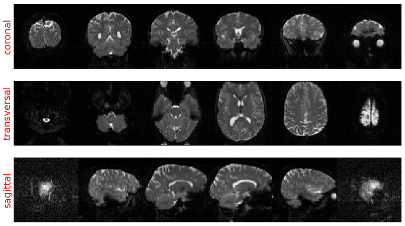
The following code will rearrange the data according to the 3 principal anatomical planes: coronal, transversal and sagittal.

 _# Orgaize the data for visualisation in the coronal plane_  
 >>> coronal = np.transpose(data_all, [1, 3, 2, 0])  
>>> coronal = np.rot90(coronal, 1)  

 _# Orgaize the data for visualisation in the transversal plane_  
 >>> transversal = np.transpose(data_all, [2, 1, 3, 0])  
>>> transversal = np.rot90(transversal, 2)  

 _# Orgaize the data for visualisation in the sagittal plane_  
 >>> sagittal = np.transpose(data_all, [2, 3, 1, 0])  
>>> sagittal = np.rot90(sagittal, 1)

After this re-organisation step we can plot the data with Matplotlib. However keep in mind that now we have a 4th time dimension which we cannot represent in a 2D image. Therefore we just look at the first timepoint. The following code can be used to visualize any slice within the coronal plane.

plt.imshow(coronal[:, :, slice_number, 0], cmap='gray')  
plt.show()

Doing this for 6 slices from each anatomical plane gives us something like the image below (code is here). You can see that no matter which way we turn the data we always get an undistorted image due to the same length of each spatial dimension.

The temporal dimension of fMRI data

Finally let’s have a look on the temporal domain. This is a bit trickier in terms of visualization since this time the result will not be a nice image of the brain, plus the amount of data points is simply too much to put into one graph; 64 x 64 x 64 x 96 = 25165824 data points. Also, we don’t know where something interesting is happening, most of the signal traces will actually show no responses to the auditory stimulation during the scan. So, the only thing we can do at the moment is to pick any random voxel in any of the slices and plot its time course.

 _# Create an empty plot with defined aspect ratio_  
 >>> fig, ax = plt.subplots(1, 1, figsize=[18, 5])  

 _# Plot the timecourse of a random voxel_  
 >>> ax.plot(transversal[30, 30, 35, :], lw=3)  
>>> ax.set_xlim([0, transversal.shape[3]-1])  
>>> ax.set_xlabel('time [s]', fontsize=20)  
>>> ax.set_ylabel('signal strength', fontsize=20)  
>>> ax.set_title('voxel time course', fontsize=25)  
>>> ax.tick_params(labelsize=12)  

>>> plt.show()

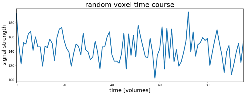
Well it is a time course, right? It neither looks very meaningful nor does it seem to carry much information about what is going on in the brain during the scan. In order to get more insights out of fMRI data we actually need to put some more effort into analyzing the temporal dimension of the data. But since this cannot be coded or explained in two or three lines we will have a look at this topic in the next post.

Meanwhile you can check out the complete code here, follow me on Twitter or connect via LinkedIn.

The code for this project can be found on Github.