Biological neural networks such as the human brain consist of specialized cells called neurons. There are various types of neurons but all of them are based on the same concept. Signaling molecules…

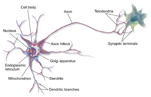
Biological neural networks such as the human brain consist of specialized cells called neurons. There are various types of neurons but all of them are based on the same concept. Signaling molecules called neurotransmitters are released at the synapse, the connection point between two neurons. Neurotransmitters alter the membrane potential of the post-synaptic cell by interacting with ion channels within their cellular membrane. If the depolarization of the post-synaptic cell is strong enough an action potential is generated at the axon hillock. The action potential will travel along the axon and trigger the release of neurotransmitters into the synaptic cleft which will affect the membrane potential of the next neuron. This way a signal can be passed on from one cell to the next through the (entire) network with the action potential being the trigger for the release of neurotransmitters at the synapse. Neural communication is electro-chemical in nature and knowing when and under which conditions action potentials are generated can give valuable insights into the workings of the brain.

By BruceBlaus [CC BY 3.0 (https://creativecommons.org/licenses/by/3.0)], from Wikimedia Commons

But studying the activity of individual neurons inside the living brain is a challenging task. There is no non-invasive method available through which neural activity can be monitored on a single cell level in real time. Usually an electrode is inserted into the brain to record the electrical activity in its near vicinity. In these kind of electrophysiological recordings an action potential appears as a fast high amplitude spike. But because neurons are densely packed inside the brain a recording electrode will typically pick up spikes from more than just one neuron at a time. So if we want to understand how individual neurons behave we need to extract the spikes from the recording and check if they were generated by one or potentially several neurons. Extracting and clustering spikes from the data is referred to as spike sorting. In the following we will outline the process of extracting individual spikes from raw data and preparing them for spike sorting.

Getting started

So first we need data. There is a popular spike sorting algorithm available for Matlab called Wave Clus. In the data section of their web page they provide a test dataset which we will use here. According to the information provided on the web page the recording is about 30 minutes long and comes from an epilepsy patient. The data is stored in an . ncs file which is the data format of the company that manufactured the recording system. So if we want to read the recording into Python we need to understand how the data is stored. There is a detailed description about the  .ncs file format on the companies web page which we can use to import the file:

>>> # Define data path  
>>> data_file = './UCLA_data/CSC4.Ncs'


>>> # Header has 16 kilobytes length  
>>> header_size   = 16 * 1024


>>> # Open file  
>>> fid = open(data_file, 'rb')


>>> # Skip header by shifting position by header size  
>>> fid.seek(header_size)


>>> # Read data according to Neuralynx information  
>>> data_format = np.dtype([('TimeStamp', np.uint64),  
>>>                         ('ChannelNumber', np.uint32),  
>>>                         ('SampleFreq', np.uint32),  
>>>                         ('NumValidSamples', np.uint32),  
>>>                         ('Samples', np.int16, 512)])


>>> raw = np.fromfile(fid, dtype=data_format)


>>> # Close file  
>>> fid.close()


>>> # Get sampling frequency  
>>> sf = raw['SampleFreq'][0]


>>> # Create data vector  
>>> data = raw['Samples'].ravel()

As we can see in the above code the  .ncs file also contains some additional information about the recording. Most importantly, the sampling frequency which tells us how many data points were recorded per second. With the sampling frequency and the number of samples in the data we can now create a time vector which allows us to plot the signal over time. The following code will do this and plot the first second of the signal.

>>> # Determine duration of recording in seconds  
>>> dur_sec = data.shape[0]/sf


>>> # Create time vector  
>>> time = np.linspace(0, dur_sec,data.shape[0])


>>> # Plot first second of data  
>>> fig, ax = plt.subplots(figsize=(15, 5))  
>>> ax.plot(time[0:sf], data[0:sf])  
>>> ax.set_title('Broadband; Sampling Frequency: {}Hz'.format(sf), >>>               fontsize=23)  
>>> ax.set_xlim(0, time[sf])  
>>> ax.set_xlabel('time [s]', fontsize=20)  
>>> ax.set_ylabel('amplitude [uV]', fontsize=20)  
>>> plt.show()

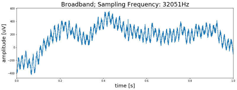
Alright, so do we see spikes? … No we don’t. But we do see some kind of rhythmic activity in the data. So is this a meaningful signal? Again the answer is no. If we were to count the number of peaks in this first second of data we would end up with a count of 60 peaks, meaning we are looking at a 60 Hz oscillation. We can further confirm this by plotting the power spectrum of the signal which shows a clear peak at 60 Hz.

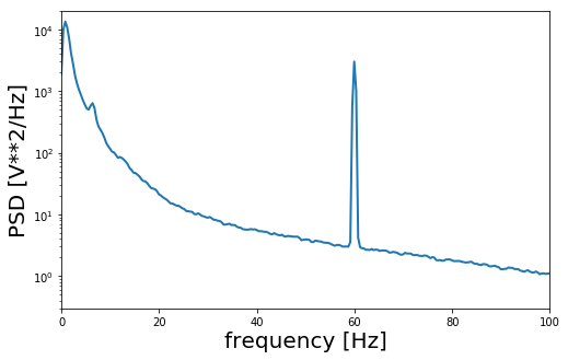
So what are we looking at? On the web page where we got the data from it says that the recording is coming from Itzhak Fried’s lab at UCLA in he US. The power supply frequency in the United States is 60 Hz. So what we are looking at is actually electrical noise from the electronic devices that were in the room during the data collection.

Finding the spikes in the signal

Even though there is 60 Hz noise in the data we can still work with it. Lucky for us action potentials are fast events that only last for 1 to 2 milliseconds. So what we can do here is to filter the raw broadband signal in a range that excludes the 60 Hz noise. A typical filter setting is 500 to 9000 Hz and our Python implementation looks as follows:

>>> # Import libarys  
>>> from scipy.signal import butter, lfilter


>>> def filter_data(data, low=500, high=9000, sf, order=2):  
>>>     # Determine Nyquist frequency  
>>>     nyq = sf/2


>>>     # Set bands  
>>>     low = low/nyq  
>>>     high = high/nyq


>>>     # Calculate coefficients  
>>>     b, a = butter(order, [low, high], btype='band')


>>>     # Filter signal  
>>>     filtered_data = lfilter(b, a, data)  
>>>      
>>>     return filtered_data

Processing the data with the above function will give us the high frequency band, or spike channel, of the signal. Our expectation is that this spike channel contains the action potentials and has no 60 Hz noise anymore. So lets look at the filtered spike channel and compare it to the raw broad band signal.

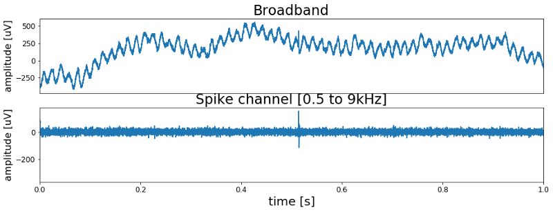
As expected the spike channel shows no 60 Hz oscillation anymore. And most importantly we finally can see the first spike in the recording. Around 0.5 seconds into the recording it is clearly visible in the filtered data. Also, now that we now where to look, we can see it in the unfiltered data. However it is harder to spot because of the 60 Hz noise.

Extracting spikes from the signal

Now that we separated the high frequency spike band from the noisy low frequency band we can extract the individual spikes. For this we will write a simple function that does the following:

1. Find data points in the signal that are above a certain threshold
2. Define a window around these events and “cut them out”
3. Align them to their peak amplitude

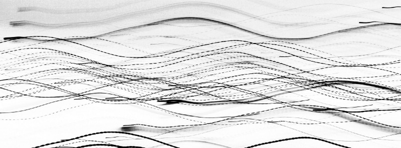
Additionally we will also define an upper threshold. Data points above this threshold will be rejected as they are likely high frequency artifacts. Such artifacts may arise through movements of the patient or might reflect electrical events like switching on or off a light bulb in the room. You can have a detailed look at the spike extraction function in the Jupyter Notebook. Here we will just have a look at 100 random spikes that were extracted form the signal with our function.

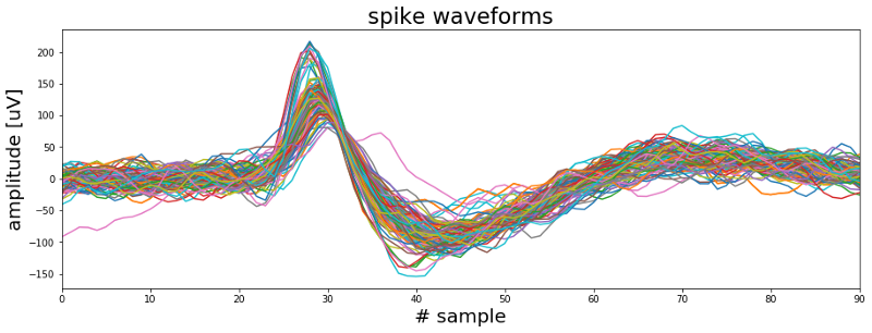
In the above plot we can see that there are at least two types of waveforms in the data. One group of spikes with a sharp high amplitude peak and a second group with a broader initial peak. So most likely these spikes were generated by more than one neuron. The next task therefore is to find a way to group the waveforms into different clusters. But since this cannot be coded or explained in two or three lines we will have a look at the spike sorting topic in the next post.

Meanwhile you can check out the complete code here, follow me on Twitter or connect via LinkedIn.

The code for this project can be found on Github.