My grandmother was an outstanding cook. So when I recently came across her old cook book I tried to read through some of the recipes, hoping I could recreate some of the dishes I enjoyed as a kid. However this turned out harder than expected since the book was printed around 1911 in a typeface called f raktur.

My grandmothers cook book meets machine learning part I

Figure 1: My grandmothers old, German cookbook: _” Praktisches Kochbuch” by Henriette Davidis

Unfortunately the fraktur typeface deviates from modern typefaces in several instances. For example the letter ” A” looks like a ” U” in fraktur and every time I see a ” Z” in fraktur I read a ” 3” (see Figure 2).

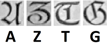Figure 2: Examples of letters in fraktur and in a modern typeface (Calibri)

So the idea emerged to develop a pipeline that will create a live translation of the fraktur letters into a modern typeface. With such a tool in hand we could easily read through the recipes and focus on the cooking part instead of deciphering the book. Luckily there are many great open source tools out there that will help us to develop such a pipeline. However some aspects of this project have to be build from scratch. Mainly we need a dataset to train our machine learning algorithm(s) on. And this is what we will focus on in this article. But before we get started with the dataset, lets have a quick look on all the tasks that lay ahead of us:

1. Detect individual letters in an image
2. Create a training dataset from these letters
3. Train an algorithm to classify the letters
4. Use the trained algorithm to classify individual letters (online)

We will cover the first two topics within this article and continue on topics 3 and 4 in a second and third article. This should give us enough room to explore each of the tasks in detail.

Also as a ** general remark: In these articles we will not focus on how to implement each algorithm from scratch. Instead we will see how we can connect different tools to translate the cook book into a modern typeface. If you are more interested in the code than in the explanations you can also go directly to the Jupyter Notebooks on Github.

Detecting letters in an image

So the first task is finding a way to extract individual letters from the pages of the cook book. This is the basis for everything that follows. In the next step we can then create a dataset from the extracted letters and finally train a classifier on it.

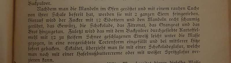Figure 3: Picture of one paragraph of the cook book

The inputs to our pipeline will always be pictures of pages from the cook book similar to the one shown in Figure 3 above. These inputs can be either single high resolution images from a smartphone camera or a stream of images from a webcam. What we have to ensure is that each image, independent from its source, is processed in a way that the detection algorithm can find all single letters. The first thing to remember here is that digital cameras store images in three separate channels: R ed, G reen and B lue ( RGB ). But in our case these three channels contain redundant information as the letters can be identified in each of these three channels separately. Therefore we will convert all images to gray scale first. As a result, instead of three channels we only have to deal with one channel. In addition we also reduced the amount of data to 1/3 which should improve performance. But our detection algorithm will face another problem: varying lightning conditions. This complicates the separation of letters from the background as contrast changes across the image. To solve this we will use a technique called adaptive thresholding which uses close-by pixels to create local thresholds which are then used to binarize the image. As a result the processed image will only consist of black and white pixels; no gray anymore. We can then further optimize the image for letter detection by denoising it with a median blur filter. The code below outlines a Python function that does the image conversion from RGB to black and white with the help of the openCV library. The result of this processing step is further exemplified in Figure 4.

# Define a function that converts an image to thresholded image  
def convert_image(img, blur=3):  
    # Convert to grayscale  
    conv_img = cv2.cvtColor(img, cv2.COLOR_BGR2GRAY)


    # Adaptive thresholding to binarize the image  
    conv_img = cv2.adaptiveThreshold(conv_img, 255,     
               cv2.ADAPTIVE_THRESH_GAUSSIAN_C,   
               cv2.THRESH_BINARY, 11, 4)


    # Blur the image to reduce noise  
    conv_img = cv2.medianBlur(conv_img, blur)   

    return conv_img

Figure 4: The left image shows the original picture, middle image shows the gray scaled version and the right image shows the thresholded and blurred result.

Ok now that we processed the image it is time to detect the letters. For this we can use the findContours method of the openCV library. The code boils down to a single line which is called by the function below. We can then map the bounding boxes of the contours found by this function back onto the original RGB image to see what was actually detected (Figure 5).

# Define a function that detects contours in the converted image  
def extract_char(conv_img):  
    # Find contours  
    _, ctrs, _ = cv2.findContours(conv_img, cv2.RETR_TREE,    
                 cv2.CHAIN_APPROX_SIMPLE)


    return ctrs

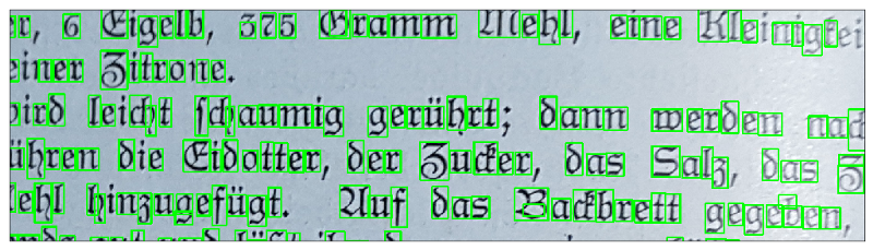Figure 5: Result of detected contours mapped back onto the original image.

From Figure 5 we can see that the detection works quite well. However in some cases letters are not detected, e.g. some of the ” i”_s at the end of line 1. And in other cases a single letter is split into two letters, e.g. _” b” at the end of the last line. Another thing to notice is that some letter combinations essentially become a single letter and are detected accordingly by the algorithm, two examples from Figure 5 are ” ch” and ” ck”. We will later see how to deal with these issues. But for now we can move on with the current result. So since we have the bounding boxes of each letter we can cut them out and save them as individual images (.png) in a folder on our hard drive. If you are interested in how to do this, have a look into the Jupyter Notebook.

Creating the dataset

Having a set of extracted letters is good but we need to organize them in a way that the dataset becomes useful for us. For this we have to do two things:

1. Remove images that do not contain letters. This can be artifacts of all kinds, e.g. a smear on one of the pages or only parts of a letter as we have seen in Figure 5.
2. Group all remaining images. This means all letters ” A” go into one folder, all letters ” B” go into another folder and so on.

Both of the above points are, in principle, easy to solve. However, since we extracted several thousands of potential letters from many pages of the book they pose a long and tedious task. On the bright side, we can automatize the first round of the grouping so that we will later “only” have to correct the result of this pre-grouping step. But there is one more thing to do before we can get started with this clustering step: We have to bring all images of the extracted letters to the same size.

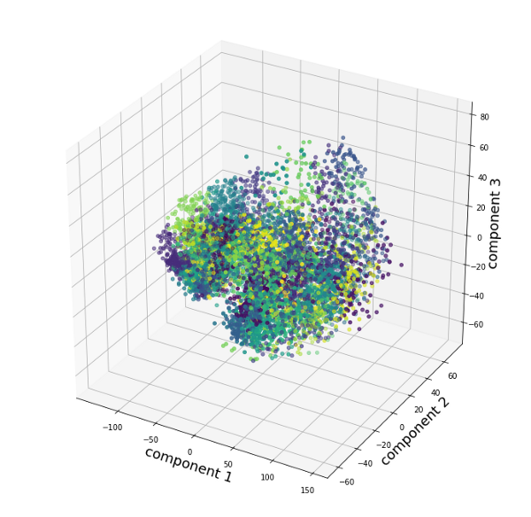Figure 6: Scatter plot of the first 3 PCA scores. Color represents the cluster.

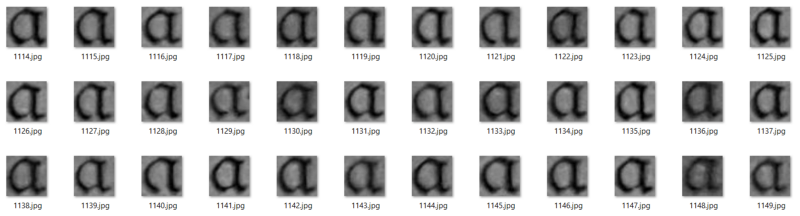
The reason for this is that the algorithms we will use for the clustering and also for the classification, expect a fixed size of the input images. But as we can see from the bounding boxes in Figure 5 each image currently has a different shape. To overcome this variety of image sizes we will use the resize method of the openCV library and bring all images to the same size. We will then store the images in a Numpy array and normalize them by calculating their z-scores. The normalization is important for the next step, which is reducing the number of dimensions of each image with Principal Component Analysis (PCA). The scores of the first principal components will then be the input to the K-Means clustering algorithm which will do the pre-clustering of the letters for us. If you are interested in the details of this procedure and the K-Means algorithm you can check either the Jupyter Notebook to this article or learn about a different use case here. The results of the K-Means clustering are visualized in Figure 6 where the color of each dot indicates the cluster it belongs to. Looking at Figure 6 __ it seems like some data points form groups that were also assigned to the same cluster by the K-Means algorithm. However, it is difficult to judge from Figure 6 alone how well the clustering worked. A better way to evaluate the results is to move all images in a cluster to a separate folder and than have a look at the content of each cluster. Figure 7 shows the images in an example folder where the clustering worked very well. The next step would be to rename this folder to “a”.

In other cases the clustering did not work so well. Figure 8 __ shows an example of a cluster that contains different types of letters. While most of the letters are “n”s there are also some “K”s and “u”s in the cluster. However we can easily fix this by searching for the “K” and “u” clusters and move the images there. Afterwards the folder can be renamed to “n”.

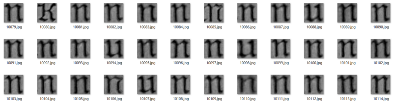Figure 8: Example folder with clustered data that contains different letters

We will continue like this until all clusters are cleaned and renamed as described above. The result should look similar to Figure 9, where upper case letters are marked by “_”.

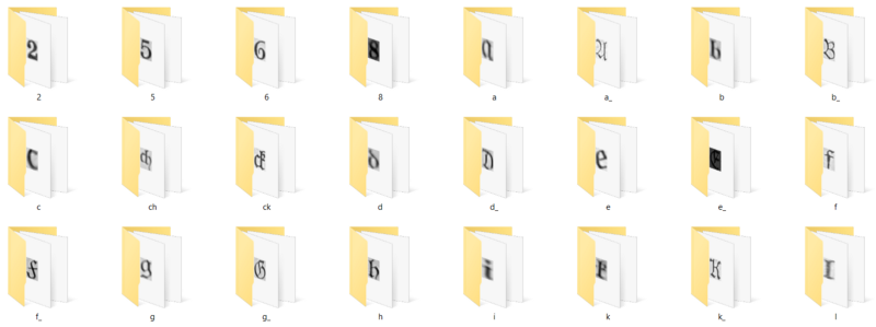Figure 9: Example of how the data should be organized after clustering and manual adjustments.

So, obviously it needed some manual work to get the data into shape. However we were able to automatize a big part of the work by pre-clustering the data with PCA and K-Means. The dataset is now cleaned and organized, but for us to work efficiently we need to save it in a more convenient way than folders on the hard drive.

Converting the dataset to the IDX format

The final step, to wrap all of this up is therefore to convert the dataset into the IDX data format. You might be familiar with this format already as the famous MNIST dataset is saved in the same way. Only here instead of reading the data from an IDX file we have to write it.
We will do so by using an idx_converter which takes a file structure as we set up above and directly saves it in the IDX format. The output will be two files: one file with the images and a second file with the labels.
Since we want to later train a classifier on the data, we should already split the images into a training and a test dataset. For this we will move 30% of the letters to a test folder while the remaining letters stay in the training folder. You can check the code in the Jupyter Notebook for details about the implementation of this procedure.

Now that we created a fraktur dataset from scratch we can move on to the next article in which we will compare the performance of several classifier algorithms in order to select one for the live translation of the cook book.

Meanwhile you can check out the complete code for this article here, follow me on Twitter or connect via LinkedIn.