It has been a long standing task to create machines that can act and reason in a similar fashion as humans do. And while there has been lots of progress in artificial intelligence (AI) and machine learning in recent years some of the groundwork has already been laid out more than 60 years ago. These early concepts drew their inspiration from theoretical principles of how biological neural networks such as the human brain work.

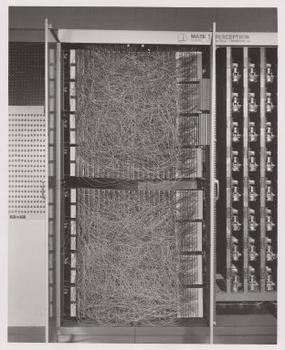Hardware implementation of the Perceptron (Mark I)

A biologically inspired linear classifier in Python

In 1943 McCulloch and Pitts published a paper describing the relationships of (artificial) neurons in networks based on their “all-or-none” activity characteristic. This “all-or-none” characteristic refers to the fact that a biological neuron either responds to a stimulation or remains silent, there is no in between. A direct observation of this behavior can for example be seen in micro electrode recordings form the human brain. After this initial paper on artificial neural networks Frank Rosenblatt in 1957 published a paper entitled “The Perceptron – A Perceiving and Recognizing Automaton”. The Perceptron is a supervised linear classifier that uses adjustable weights to assign an input vector to a class. Similar to the 1943 McCulloch and Pitts paper the idea behind the Perceptron is to resemble the computations of biological neurons to create an agent that can learn. In the following we will have a look on the idea behind the Perceptron and how to implement it in Python code.

The idea

Your brain contains billions of neurons and each of them can be seen as a processing unit that integrates inputs and creates a binary response based on a threshold criterion. In biological terms the inputs are membrane depolarizations at the dendrites of the neuron which spread towards the soma. If the depolarization is strong enough the neuron will respond by generating an action potential which will travel along the axon. At the axon terminal neurotransmitters will be released into the synaptic cleft which will depolarize the dendrites of the downstream neuron. A more detailed description of this process can be found here. Now the actual clue is that a network of biological neurons can learn how to respond to its inputs. The term for this feature is plasticity and it is this property that makes the difference between a static piece of software and an intelligent agent that can adapt to its environment. The 1943 McCulloch and Pitts paper however did not address this issue instead it focused on the relationships among neurons. The Perceptron on the other hand offered an elegant solution for the plasticity problem: weights. ** Every input of the Perceptron gets multiplied by a weight and then the results get summed up. So by changing the weights of the inputs we can alter the Perceptrons response. The figure below gives a schematic overview of how the Perceptron operates.

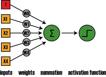Figure 1: Schematic outline of the Perceptron

On the left hand side of Figure 1 the inputs are represented as x1, x2, x3,…xn. Each input gets multiplied by a weight w0, w1, w2,… wn. After this multiplication step the results get summed up and passed through an activation function. In the case of the Perceptron the activation function resembles the “all-or-none” characteristic of a biological neuron through a heaviside step function. This means that any value ≤0 will be transformed to 0 whereas any value >0 will become 1. We can write the above also as:

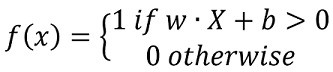
Where w is the weight vector, x is the input vector and b is a bias term. In Figure 1 we already included the bias into the input vector as a 1 (red square) and into the weight vector as w0. So in this case the dot product of the input and the weight vector is all we need to calculate. But one question remains: How do we adjust the weights? After all this is how the Perceptron learns. One way to think about this is as follows. Our Perceptron is supposed to make a binary decision (0 or 1) based on its inputs. So imagine we have two data points, one belongs to class 1 the other to class 0 and the Perceptron has to learn the class of each data point. The task is visualized in the Figure 2 below.

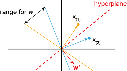!Figure 2: Geometrical interpretation

From Figure 2 we can see that the problem can be viewed as finding a decision boundary, also called hyperplane (red dashed line) , that separates the two groups. Everything above the red dotted line will be class 0 and everything below the hyperplane will be class 1. The hyperplane is defined by a weight vector w’ which is perpendicular to it (red solid vector). Therefore calculating the dot product of the input vector with the weight vector and passing the result through the activation function will give us the classification of the input. So if we take a look at data point 1 we can also draw it as a vector and perpendicular to it we can draw another hyperplane (solid yellow line). Next, looking at input vector 2 we can again draw a hyperplane perpendicular to it (solid blue line). Since the hyperplane which separates the two groups needs to be perpendicular to the weight vector we are looking for, it becomes obvious from Figure 2 that w’ has to lay between the yellow and blue hyperplanes (labeled as “range for x “). So following the above we can implement the learning rule as follows.

First we set all values in our weight vector to zero, including the bias term. In the case of a two dimensional input, like in Figure 2, this means: w = [0 0 0]. Then we add the bias of 1 to our first input vector which gives us X(1) = [1, x1, x2]. Now we calculate the dot product of X1 and w. The result of this calculation is 0. Passing 0 through the activation function will then classify X1 as class 0, which is correct. Therefore no update of w is needed. Doing the same for X(2) also gives us class 0 which is wrong so we need to update w by the following learning rule:

In this case it means subtracting our result (class 0) from the correct class (1), multiplying the outcome by the current input vector and adding it to w. This will result in: w = [1 x1, x2]. If there would be more data points we would continue with this procedure for every input vector and with every iteration we would come closer to a weight vector that describes a hyperplane which linearly separates our two groups. To test this we will next implement the Perceptron in Python code.

The Implementation

To develop our Perceptron algorithm we will use toy data which we generate with scikit-learn. All other functions we will implement using NumPy. The complete Jupyter Notebook with all the code for this article can be found here. The code below will create and visualize our toy data set.

# Import libraries   
from sklearn.datasets import make_blobs  
import matplotlib.pyplot as plt  
import numpy as np


# Generate dataset  
X, Y = make_blobs(n_features=2, centers=2, n_samples=1000, random_state=18)


# Visualize dataset  
fig, ax = plt.subplots(1, 1, figsize=(5, 5))  
ax.scatter(X[:, 0], X[:, 1], c=Y)  
ax.set_title('ground truth', fontsize=20)  
plt.show()

Figure 3: Data for testing the Perceptron algorithm.

Figure 3 shows the two clusters we just created and as we can see they can be linearly separated by a hyperplane, the precondition for the Perceptron to work. Next we need to add the bias term to the input vector and initialize the weight vector with zeros.

# Add a bias to the X1 vector  
X_bias = np.ones([X.shape[0], 3])  
X_bias[:, 1:3] = X


# Initialize weight vector with zeros  
w = np.zeros([3, 1])

OK now we are all set to code the Perceptron algorithm. As we can see from the code below it is a strikingly simple and elegant algorithm. Because it is not guaranteed that the Perceptron will converge in one pass, we will feed all the training data into the Perceptron 10 times in a row while constantly applying the learning rule, just to make sure.

# Define the activation function  
def activation(x):  
    return 1 if x >= 1 else 0


# Apply Perceptron learning rule  
for _ in range(10):  
    for i in range(X_bias.shape[0]):  
        y = activation(w.transpose().dot(X_bias[i, :]))


        # Update weights  
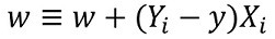
        w = w + ((Y[i] - y) * X_bias[i, :]).reshape(w.shape[0], 1)

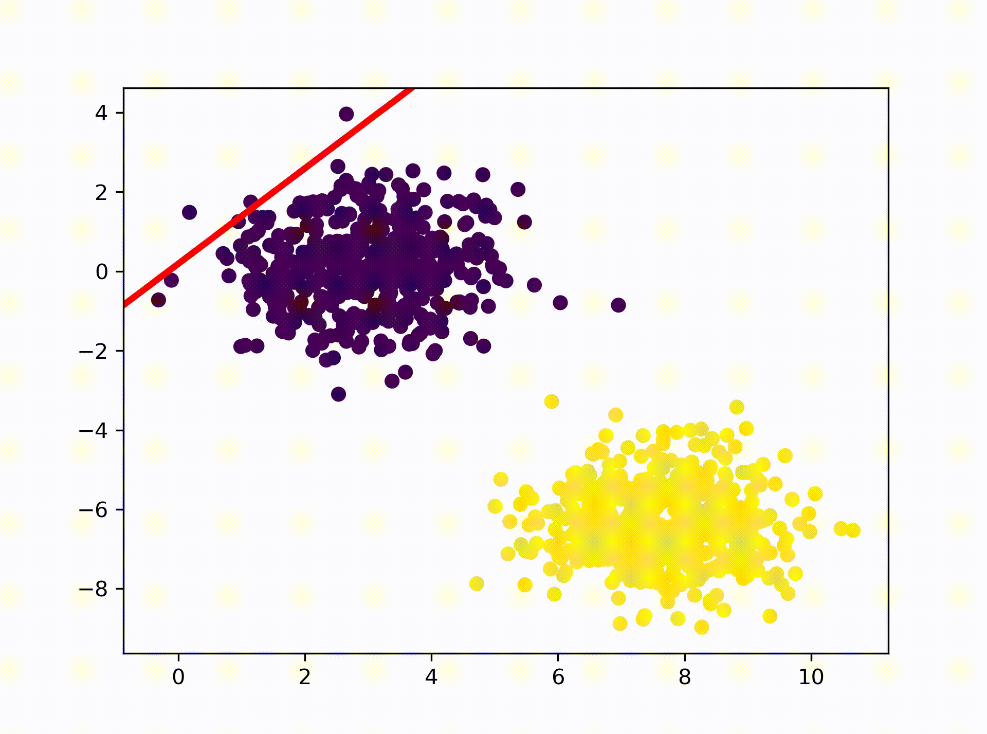
So lets have a look at the result. The animation below visualizes how the Perceptron is searching for a hyperplane that separates the two clusters. As we can see it eventually comes up with a solution where one of the class 1 data points lays on the hyperplane. That solution is actually correct as we specified earlier in our activation function: return 1 if x >= 1 else 0 If you are interested you can re-run the above code with the the following activation function to see how the result changes: return 0 if x <= 0 else 1

Conclusion

Finally, before we finish some thoughts on the above. As we saw the Perceptron algorithm is a simple way of implementing a supervised linear classifier. However it also has drawbacks. For example it does not work when the groups are not linearly separable. Also it is an online algorithm which means we can only pass one training example at a time into it, making the training process slow if we had a larger dataset. Despite these limitations the Perceptron actually is an important concept that started the first AI hype. Ironically it also ended it a couple of years later when it couldn’t fulfill the big promises that were made about it.

If you want the complete code of this project you can find it here. And of course feel free to follow me on Twitter or connect via LinkedIn.